1.- Introduction Link to heading
This post is about steganographic tools and analysis techniques in search of hidden information. In this case, the S-Tools tool is used. We will also use a custom python script to help us analyze the images bit by bit in search for hidden information. Lastly, we will also perform a histogram analysis, coding another custom python script.
S-Tools is a very powerful tool developed by Andy Brown. It allows you to hide messages using steganography in BMP, GIF, and WAV images. It is a very simple tool that allows drag-and-drop to process the relevant files. Additionally, it can encrypt the hidden information so that even if the message is discovered, the information cannot be decrypted without the password.
The program selects the bits it modifies using a pseudo-random algorithm, making it difficult to discover and/or extract the message. This fact is discussed in detail later, when we attempt to examine the suspicious image using color and histogram analysis.
2.- Extraction of the hidden message using S-Tools Link to heading
By dragging the photograph into the S-Tools.exe program window, right-clicking, and selecting “Reveal…,” the password is then entered, and the program extracts the information, which can be saved to the hard drive. In this case, it is six text files:
Illustration 1: Hidden Files Revealed
3. Questions Link to heading
3.1- How many bytes of information have been hidden in the image? Link to heading
A total of 734891 bytes (717 KB) have been hidden, spread over a total of 6 text documents.
Illustration 2: Hidden files.
Illustration 3: Total size of the hidden files.
3.2- What is the insertion ratio? Link to heading
To calculate the insertion ratio, the following formula is used:
$$ Insertion\ Ratio = \frac{Size\ of\ hidden\ bytes}{Size\ of\ total\ image} $$
The insertion ratio in this case is 0.31148, or 31.1%. This is a fairly high insertion ratio, so the difference between the original image and the modified image can be noticed at a glance, i.e. it has a low transparency.
3.3- Is there a significant difference between the disk space of the original image and the one with the hidden message? Link to heading
There is no significant difference between the disk space of the original image and the one with the hidden message. There is a negligible difference of two bytes between them and, in fact, the original image occupies slightly more space than the processed image.
Illustration 4: Difference in size between the original image and the modified image.
We are talking about a difference of a couple of bytes, insignificant. This makes sense since the LSB technique is used, in which no “extra” bits of information are added, but the least significant bits of each pixel are modified.
3.4- Open the two images with GIMP and compare the value of a group of pixels, can you state the insertion method? Explain what the difference is Link to heading
Let’s examine the upper left pixel. To do this, we import the images into GIMP and with the Colour Picker tool we can check the RGB value of the chosen pixel.
Illustration 5: RGB values of the upper pixel of the modified image.
This pixel of the modified image has the RGB values [212, 224, 228] and the HEX value 0xd4e0e4.
Illustration 6: RGB values of the upper pixel of the original image.
This pixel of the original image has the RGB values [217, 228, 231] and the HEX value d9e4e7. The binary values of these pixels are as shown in the following table:
| Original Pixel (DEC) | Original Pixel (BIN) | Modified Pixel (DEC) | Modified Pixel (BIN) | |
|---|---|---|---|---|
| R Channel | 217 | 11011001 | 212 | 11010100 |
| G Channel | 228 | 11100100 | 224 | 11100000 |
| B Channel | 231 | 11100111 | 228 | 11100100 |
It can be seen that even the fourth least significant bit is modified. By modifying more bits of each color, more information can be hidden. However, the quality of the image is affected, so it is easier to see that the image has been altered in some way. In this case, the difference between the original image and the image with the hidden message is clearly noticeable, so it has a low transparency or imperceptibility.
4.- Image analysis Link to heading
4.1- Visual analysis of LSB-Replacement Link to heading
It is sometimes possible to identify with the naked eye if the image has been modified. This is achieved by magnifying the image pixels to visually detect if information is being hidden.
Illustration 7: Original image vs modified image. Image obtained from the course notes.
A Python script has been written that sets the bytes with LSB1 to 0 and the bytes with LSB 0 to 255, resulting in the following image:
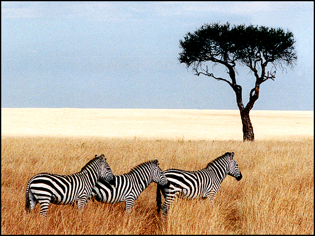
Illustration 8: Image with hidden information.
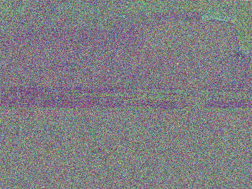 Illustration 9: Image after script processing.
Nothing is visible to the naked eye. This is because the S-Tools program uses up to 4 bits from the end of each color byte, so by processing only the end bit nothing suspicious is found. The same analysis has also been tried with the second least significant bit and with the third one:
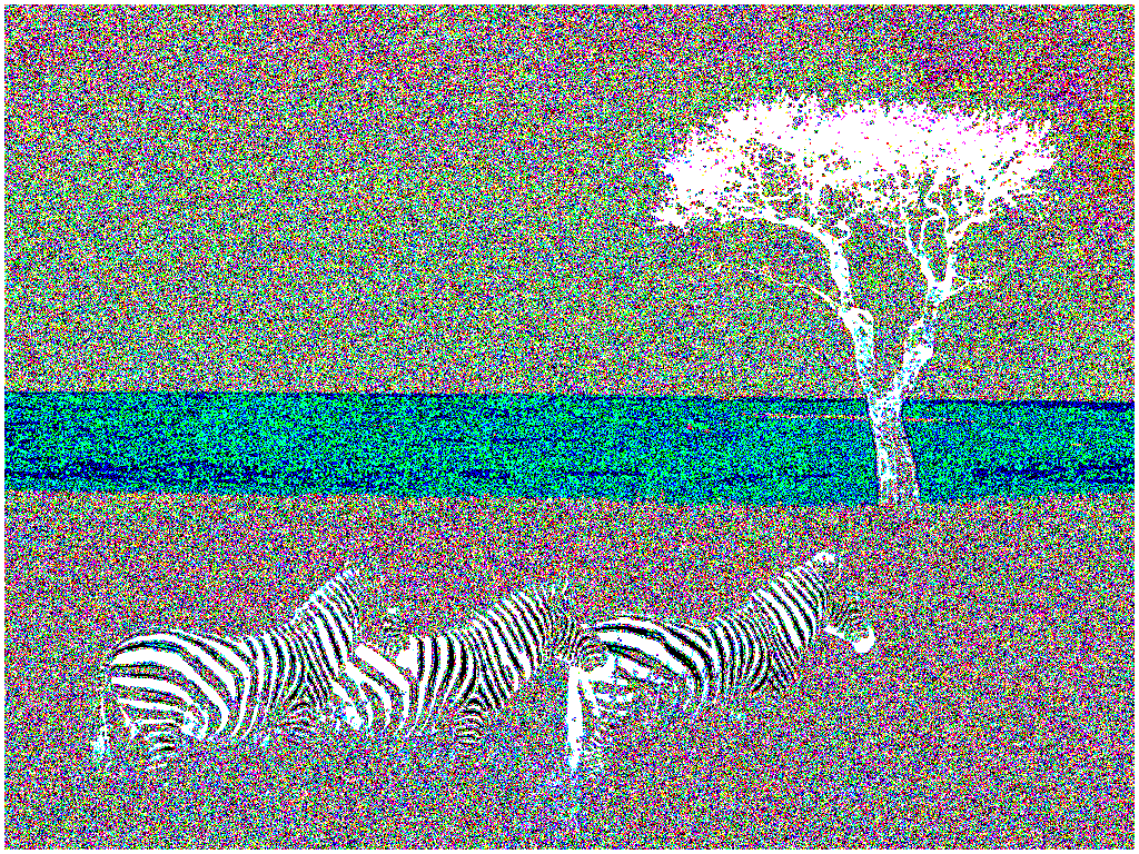
Illustration 10: Treatment of the second significant bit.
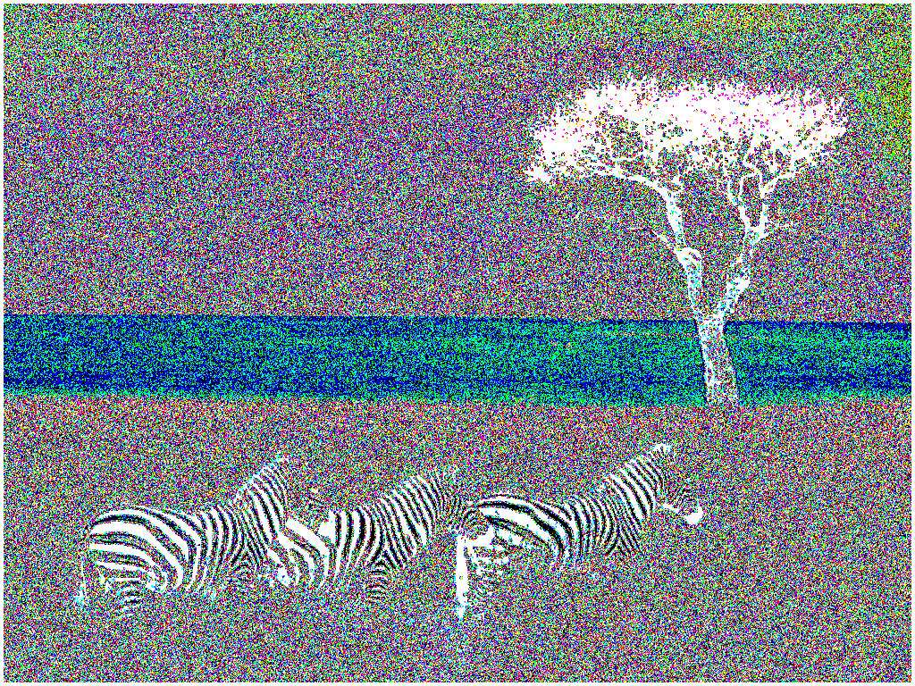
Illustration 11: Treatment of the third significant bit.
Nothing excessively obvious can be seen either, so the S-Tools program’s way of hiding messages is very robust.
4.2- Histogram analysis Link to heading
By means of a histogram analysis it is possible to detect the existence of hidden information. This is because LSB-Replacement techniques tend to “equalize” the number of times each color appears even or odd. This means that, if there is hidden information, the histogram bars are matched two to two. To analyze the occurrence of this event, a Python script has been developed that counts the number of occurrences of each RGB value, per channel in this case.
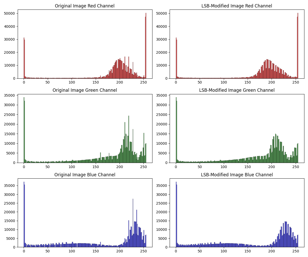
Illustration 12: Comparison between the histograms of the original image and the image with hidden information.
It can be clearly seen that there is a difference between the histograms. Apparently, the S-Tools algorithm “clips” some of the frequency peaks and uses them to hide the information. If you zoom in, you can see something interesting.
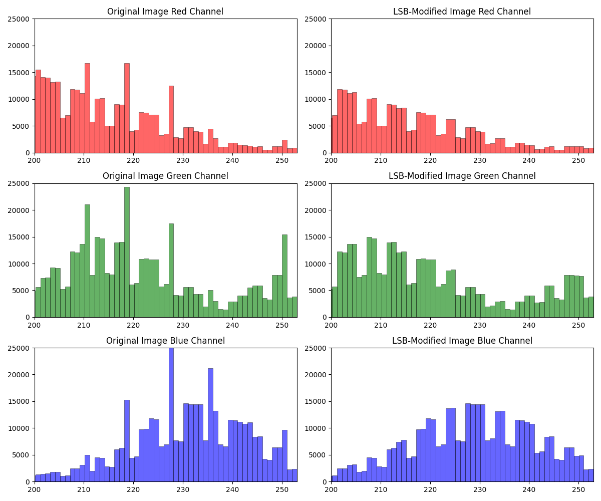
Illustration 13: Zoom of the histogram, between sample 200 and 254.
You can see that the odd and even histogram bars look very similar to each other. This is quite strong evidence that the image contains hidden information. It is interesting that this phenomenon occurs, since in this case the information is encoded in the last 4 bits of each RGB channel of each pixel, not only in the last one. Nevertheless, this phenomenon may indicate that there is a hidden message, and that the image needs to be further analyzed.
Conclusion Link to heading
The S-Tools.exe program is a fairly robust steganographic information hiding program. It has passed the color and histogram analysis with no obvious indications of hidden information, so it is very robust. The capacity is very high, with an insertion rate of more than 30% in this case. In terms of transparency, and given the high capacity, a significant number of bits are modified in each pixel, so the image is clearly altered. This makes informed detection relatively straightforward. However, blind detection is somewhat more complicated, as seen when attempting to analyze it using color modification techniques and histogram analysis.
6.- Code Link to heading
6.1- Code og color_analysis.py Link to heading
from PIL import Image

import numpy as np

def load_image(file_path):

    # Open the image using Pillow

    image = Image.open(file_path)

    # Ensure image is in RGB format

    image = image.convert("RGB")

    # Convert image to a Numpy array

    img_array = np.array(image)

    return img_array

def apply_LSB_operation(image_array):

    # Get image dimensions (height, width)

    height, width, _= image_array.shape

    # Process each pixel

    for y in range(height):

        for x in range(width):

            r, g, b = image_array\[y, x\]

            # Apply LSB operation to Red channel

            if r % 2 == 1:  # If LSB of Red is 1

                r = 0

            else:           # If LSB of Red is 0

                r = 255

            # Apply LSB operation to Green channel

            if g % 2 == 1:  # If LSB of Green is 1

                g = 0

            else:           # If LSB of Green is 0

                g = 255

            # Apply LSB operation to Blue channel

            if b % 2 == 1:  # If LSB of Blue is 1

                b = 0

            else:           # If LSB of Blue is 0

                b = 255

            # Update the pixel with the new values

            image_array\[y, x\] = (r, g, b)

    return image_array

def save_image(image_array, output_path):

    # Convert Numpy array back to image

    output_image = Image.fromarray(image_array)

    # Save the image

    output_image.save(output_path)

def main():

    try:

        original_image_path = "original-zebras.bmp"     # Original image path

        output_image_path = "modified_zebras.bmp"       # Path for saving the modified image

        # Load the image as a Numpy array

        original_image_array = load_image(original_image_path)

        # Apply the LSB operation

        modified_image_array = apply_LSB_operation(original_image_array)

        # Save the modified image

        save_image(modified_image_array, output_image_path)

    except Exception as e:

        print("An error occurred:", e)

if \__name__ == "\__main_\_":

    main()
6.2- Code of histogram_analysis.py Link to heading
import numpy as np

from PIL import Image

import matplotlib.pyplot as plt

def load_image(file_path):

    # Open the image using Pillow

    image = Image.open(file_path)

    # Ensure image is in RGB format

    image = image.convert("RGB")

    # Convert image to a Numpy array

    img_array = np.array(image)

    return img_array

def plot_histograms(original_image_array, modified_image_array, output_path):

    # Create a figure with subplots

    fig, axes = plt.subplots(3, 2, figsize=(12, 10))

    # Extract the individual color channels (RGB) from both images

    original_red = original_image_array\[:, :, 0\]

    original_green = original_image_array\[:, :, 1\]

    original_blue = original_image_array\[:, :, 2\]

    modified_red = modified_image_array\[:, :, 0\]

    modified_green = modified_image_array\[:, :, 1\]

    modified_blue = modified_image_array\[:, :, 2\]

    # Range for histogram

    bins_range = 256      #All possible values


    # Plot histograms for the original image

    axes\[0, 0\].hist(original_red.ravel(), bins=bins_range, color='r', alpha=0.6, edgecolor='black', linewidth=0.5)

    axes\[0, 0\].set_title('Original Image Red Channel')

    # axes\[0, 0\].set_ylim(\[0, 25000\])

    # axes\[0, 0\].set_xlim(\[200, 253\])     # By modifying xlim, we can zoom in the image

    axes\[1, 0\].hist(original_green.ravel(), bins=bins_range, color='g', alpha=0.6, edgecolor='black', linewidth=0.5)

    axes\[1, 0\].set_title('Original Image Green Channel')

    # axes\[1, 0\].set_ylim(\[0, 25000\])

    # axes\[1, 0\].set_xlim(\[200, 253\])

    axes\[2, 0\].hist(original_blue.ravel(), bins=bins_range, color='b', alpha=0.6, edgecolor='black', linewidth=0.5)

    axes\[2, 0\].set_title('Original Image Blue Channel')

    # axes\[2, 0\].set_ylim(\[0, 25000\])

    # axes\[2, 0\].set_xlim(\[200, 253\])

    # Plot histograms for the modified image

    axes\[0, 1\].hist(modified_red.ravel(), bins=bins_range, color='r', alpha=0.6, edgecolor='black', linewidth=0.5)

    axes\[0, 1\].set_title('LSB-Modified Image Red Channel')

    # axes\[0, 1\].set_ylim(\[0, 25000\])

    # axes\[0, 1\].set_xlim(\[200, 253\])

    axes\[1, 1\].hist(modified_green.ravel(), bins=bins_range, color='g', alpha=0.6, edgecolor='black', linewidth=0.5)

    axes\[1, 1\].set_title('LSB-Modified Image Green Channel')

    # axes\[1, 1\].set_ylim(\[0, 25000\])

    # axes\[1, 1\].set_xlim(\[200, 253\])

    axes\[2, 1\].hist(modified_blue.ravel(), bins=bins_range, color='b', alpha=0.6, edgecolor='black', linewidth=0.5)

    axes\[2, 1\].set_title('LSB-Modified Image Blue Channel')

    # axes\[2, 1\].set_ylim(\[0, 25000\])

    # axes\[2, 1\].set_xlim(\[200, 253\])

    # Adjust layout

    plt.tight_layout()

    # Save the plot as a PNG file

    plt.savefig(output_path, format='png')

    # Show the plot

    plt.show()

def main():

    try:

        original_image_path = "original-zebras.bmp"     # Original image path

        modified_image_path = "zebras.bmp"              # LSB-modified image path

        output_image_path = "histogram.png"             # Histogram output path

        # Load the original and modified images as Numpy arrays

        original_image_array = load_image(original_image_path)

        modified_image_array = load_image(modified_image_path)

        # Plot histograms for comparison

        plot_histograms(original_image_array, modified_image_array, output_image_path)

    except Exception as e:

        print("An error occurred:", e)

if \__name__ == "\__main_\_":

    main()